I got to thinking recently, about the difference between the GIF and JPEG image formats: why is it that some images are larger on disk when saved as GIF, while others are larger as JPEG? It turns out that the different image formats use different methods of compression.
Compression is simply the name for a set of procedures, that allow data to be packed into a smaller space, and yet allow the data to be retrieved from the compressed encoding. It's a two-way process: an input file can yield compressed output, but putting the compressed output back into the algorithm should give you a copy of the input.
Redundancy: Run-Length Encoding
The concept that makes compression possible is redundancy: the fact that most data repeats itself in some fashion. A document may use the same word many times, for example, or a picture will contain the same colour in many places. A very simple example of a redundant piece of data could be something like the following.
Redundancy: Before compression
AAAAABBWWWWWWWWWPPPPQZMMMMVVV
In this case, the redundancy is obvious; repeated series of letters present themselves throughout the sample. An easy way to compress this would be to represent the repeated letters by the number of repeats, thus cutting down on the total length of the sample.
Redundancy: After compression
A5B2W9P4Q1Z1M4V3
An algorithm reading this encoded version of the sample will be able to perfectly retrieve the original data: "A" five times, "B" twice, and so on. This simple algorithm is used extensively, and is called run-length encoding (RLE): writing down how long each run of characters is. An example of a widely used standard employing RLE is the venerable PCX image format.

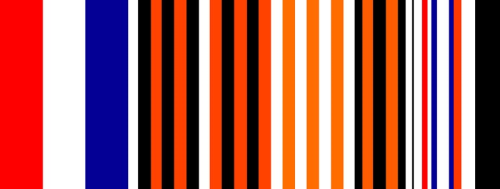
In Figure 1, there are many solid blocks of single colours. This image is 500 pixels wide, and 190 high; as a raw bitmap, using one byte to represent a pixel, this image would constitute 95kB of data. The PCX algorithm calculates run lengths for each line of pixels in the image, and then saves the run length for consecutive pixels of the same colour: in this way, the size of the image is reduced to 52kB.
Frequency: Huffman Encoding
One of the major problems with RLE is that it acts on consecutive values of data: in Figure 1, the RLE algorithm will treat each horizontal line of the image separately, whereas all the lines are the same as each other. This can be alleviated by looking at the data in the whole, and building a table of how often each value occurs in the entire data set.
Huffman encoding is a method of using this "frequency table", which denotes the frequency of occurrence for each value, and assigning each entry a code. The most frequent entries are given shorter codes, and rarer entries are relegated to receiving long codes. In computing, these codes are invariably binary codes, which can then be combined into bytes for file storage.
Using the example above, a sample Huffman encoding process may run as follows:
Huffman encoding: Before compression
AAAAABBWWWWWWWWWPPPPQZMMMMVVV
| Value | Frequency | Code |
|---|---|---|
| Q | 1 | 000000 |
| Z | 1 | 000001 |
| B | 2 | 00001 |
| V | 3 | 0001 |
| P | 4 | 001 |
| M | 4 | 011 |
| A | 5 | 01 |
| W | 9 | 1 |
Huffman encoding: After compression
01 01 01 01 01 00001 00001 1 1 1 1 1 1 1 1 1 001 001 001 001 000000 000001 011 011 011 011 0001 0001 0001 UB ù$€ m±ˆ
Using Huffman encoding, the data has been whittled down from 29 characters to 10 bytes. This does not include the frequency and coding table, which has to be stored with the compressed data for it to make any sense; in this example, the frequency table is larger than the compressed data, but the size of the frequency table is negligible in most cases.
It is, of course, possible to combine RLE and Huffman encoding, performing RLE first and then running the compressed result through the Huffman algorithm. This produces especially good results on simple images: Figure 1 above can be compressed from a 95kB bitmap to a 4kB file by using the GIF file format, which combines RLE, Huffman encoding and other algorithms.
Perception: Lossy Encoding
The methods outlined above can be used to compress data in such a manner that it can be perfectly reproduced. Examples of this usage of compression include documents and software programs, where the loss or corruption of one value may render the file worthless.
In certain circumstances, a perfect reproduction of the data in question is not necessary: a close approximation is sufficient. Generally, these circumstances arise in multimedia applications: sounds beyond the range of human hearing need not be recorded, and subtleties of colour and gradient beyond the discernment of the human eye need not be reproduced.
A classic example of this is the MPEG Audio standard, which attempts to reduce the size of audio files by removing extraneous information regarding high-frequency sounds. The Layer-3 specification of this standard allows for various settings of removal, by which progressively more information will be removed from the audio sample.

Encoded with MPEG Audio Layer-3
In Figure 2 above, two waveforms are superimposed: the original song waveform in red, and a highly compressed variant overlaid in blue. The sample shown above is 1.5 seconds long; as a section in the original waveform file, this sample is stored using 160kB of data. The compressed variant shown is of the same length, occupying only 48kB of space.
This has been achieved by the MPEG Audio compression algorithm, by transposing the sound into its frequency components, and removing those components beyond the range of human hearing (above approximately 20kHz). By doing this, the resultant waveform is not significantly affected, as can be seen above, and thus the compressed sound is not perceptibly different from that of the original source.
Throwing Data Away: Visual Lossy Encoding
Just as a sound file has high-frequency components that can't be discerned by the ear, a picture has high-frequency components: shades of colour that aren't different enough for the eye to distinguish, or gradients that run from black to white so quickly that there's no space for the gradient to be seen. Just as with sound, these components can be removed from a picture; this is the premise of the JPEG image format.
JPEG performs a variant of the same algorithm used in MPEG Audio, to retrieve a two-dimensional map of the frequency components contained within an image; the algorithm then proceeds to cut the components down, and recombine the image. An example of this process is shown below.

In Figure 3, an image composed of four 16x16-pixel squares is compared against the JPEG-encoded variant of the same file. A sharp change in colour or luminance is defined as an event of high visual frequency, and it is here where JPEG performs its removal. As a result, the encoded image has a lower definition to its edges, and the meeting point of the four squares is especially blurred.
The strength of JPEG is not in encoding images of sharp edges and corners, but instead in images of low visual frequency; photographs are a prime example of such.

In Figure 4, a 300x300 image of Antalya Harbour is encoded by JPEG. The original bitmap is 270kB, whereas by removal of the sharp edges and colour changes, JPEG is able to produce a 22kB image. As far as the human eye is concerned, very little has changed in the image; the features shown in the image survive intact, even if the pixels have changed somewhat.
This is the main concept behind lossy encoding: that the exact data is not as important as the information presented by the data. Using the JPEG algorithm to encode a software program would be unwise, but in cases where the information is more than the sum of the data, lossy encoding is ideal.
Perceptive Redundancy: Video Encoding
When it comes to video clips, it's possible to compress the data involved yet further, by combining the principles behind lossless and lossy encoding. The simplest and most naive method of building a video clip is to tack together consecutive pictures and refer to them as frames: the MJPEG video file format does this by treating a series of JPEG images as individual frames.
What this approach ignores is the inherent redundancy in a video clip: most of the information contained in a given frame is also in the previous frame. Only a small percentage of any particular frame is new information; by calculating where that percentage of information lies, and storing only that amount, it's possible to drastically cut down the data size of the frame.

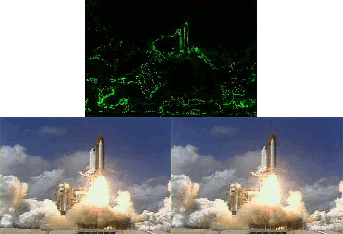
In Figure 5, the second frame of video shows very little change relative to the first: only in the Shuttle's exhaust plume is there significant motion. Indeed, the output of the SRBs and the sky behind the launch tower are entirely unchanged between frames. Instead of storing these portions of the image in their entirety, it's possible to store a single value: "No change".
The MPEG Video standard makes use of this inherent redundancy as a part of its compression algorithm. In theory, only the initial frame of a shot is required in full: any movement as part of the shot can be stored as a difference from the previous frame. The initial frame, known as an Intra-frame, is stored as a standard JPEG image, and the subsquent difference frames are called inter-frames, or Predicted frames.
In practice, the MPEG Video standard was designed with "streaming" in mind: the ability to begin viewing a video clip halfway through a shot. If only one Intra-frame (I-frame) is provided for the shot, it's not possible for the Predicted frames (P-frames) to interpolate their differences. For this reason, I-frames are commonly inserted at regular intervals into the video clip, regardless of whether a shot is in progress.

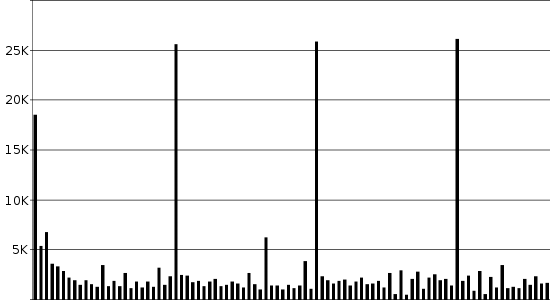
In Figure 6 above, the video clip has I-frames inserted at 25-frame intervals, or once a second. The subsequent P-frames are each much smaller in size than the I-frame, since politicians tend not to move around very much when interviewed, thus causing a lower amount of difference between frames.
The example used for Figure 6 was a 400x224 video clip of 4 seconds. In raw bitmap form, the size of the resultant file would be 26.7MB; by using the combined techniques of lossy encoding and redundancy, the MPEG Video standard is able to reduce this to 300kB, a reduction of 99%.
Conclusion: Where To Go Lossy
The examples of lossy encoding presented in this article are employed in special circumstances: audio, video, pictures. It's only in these instances, and others related to these, that perception is the important factor in the compression process. For other compression targets, such as documents and software programs, it's important to preserve the data exactly as-is.
More advanced specialisations of compression are being developed all the time, but most common implementations of compression are based on the techniques in this article: eliminating redundant and duplicate information. Compression works best when there's a lot of redundant data, so don't try to compress a compressed file.
Imran Nazar <tf@oopsilon.com>, 2008